|
Welcome to the MC-Sym FAQ. It's goal is to give
modelers hints about editing MC-Sym scripts to produce high quality
RNA 3-D structures. Each section focuses on a particular aspect of
modeling with MC-Sym, such that modelers can find easily the answers
to their questions. Here are the topics covered:
|

|
|
|
MC-Sym model (blue) superimposed on X-ray crystal structure (gold; PDB file 1EVV). The RMSD of the superposition is 4.0 Angstroms.
|
References & Links:
- Parisien M, Major F. Nature. (2008) 452:51-55.
(pubmed)
(Nature)
- The MC-Sym web page
- Dr. Francois Major's email: major at iro.umontreal.ca
- Marc Parisien's email: parisien at iro.umontreal.ca
|
|
MY FIRST RNA 3-D STRUCTURE
|
|
Let's look at the whole process of
modeling an RNA 3-D structure from sequence. Consider the sequence
fragment 72-105 from
Haloarcula Marismortui's 23S rRNA (PDB
file 1JJ2 [1]), with nucleotide A96 mutated into U:
5'-CCAUGGGGAGCCGCACGGAGGCGAUGAACCAUGG-3'
      |    |    |    |    |    |    |
     75   80   85   90   95  100  105
• Step 1. Obtain a secondary structure.
The first step in the modeling process
is to obtain a secondary structure. Classical secondary structures,
featuring only canonical base pairs (the cWW G=C, A=U and G=U) are
difficult to model in 3-D, because of the degrees of freedom an
unpaired nucleotide has. The more base pairs a secondary structure
has, the easier it will be to project it in 3-D. Using MC-Fold [2][link], we
obtain several sub-optimal secondary structures:
      >hairpin
      CCAUGGGGAGCCGCACGGAGGCGAUGAACCAUGG
   1) (((((((((((((((....)))))))))))))))  [view]  [edit]  [submit]
   2) ((((((((((((((((..))))))))))))))))  [view]  [edit]  [submit]
   3) ((((((((((((((.(...)))))))))))))))  [view]  [edit]  [submit]
   4) ((((((((((((((...))))))...))))))))  [view]  [edit]  [submit]
   5) ((((((((((((((...)))))))...)))))))  [view]  [edit]  [submit]
   6) ((((((((((((((...)))))...)))))))))  [view]  [edit]  [submit]
   7) ((((((((((((((...))))))))...))))))  [view]  [edit]  [submit]
   8) ((((((((((((((...)))))..).))))))))  [view]  [edit]  [submit]
   9) ((((((((((((((......))))))))))))))  [view]  [edit]  [submit]
Because MC-Fold's energetical
contributions for non-canonical base pairs are approximated, and that
base triples and many non-contiguous nucleobase stackings are not even
taken into account, the solution structure (PDB file 1JJ2) is ranked
#6. This secondary structure has the correct base pairing registry to
allow for a K-turn motif [1]. The confidence on a secondary structure
can be heightened by low-resolution structure probing methods like
SHAPE [3] or enzymatic and chemical probing (see for instance
[4]). Keep MC-Fold's result web page opened for further use.
• Step 2. Model by homology known motifs.
Here, our assymetrical internal loop is
most likely a K-turn motif. What we'll do is scan the PDB for this
motif using a motif descriptor, and get actual 3-D instances of that
motif. Then, by homology modeling, we can adapt the sequence in the
3-D instances to suit the sequence we are modeling. Consider the
following MC-Search [5][link] script:
//================================================
// MC-Search script to search for K-turns
// This motif is composed of two strands; A and B
//================================================
sequence( RNA A1 NGGAN )
sequence( RNA B1 NGAAGAAN )
relation(
  A1 B8 { pairing }
  B1 A5 { pairing }
)
Running MC-Search on that script will
bring you to a web page which will display an index of files in your
working directory. Working directories, identified by unique 10-digit
keys, are used to store results from the MC-Pipeline suite of
programs. All 3-D instances which correspond to the motif descriptor
are put in the file results.pdb. The search should have
returned only one 3-D instance.
Modeling by homology for nucleic acids
necessitate two operations: 1) mutating nucleobases and 2) mutating
base pairs. These operations can be performed via the file
commands.html. In the "sequence mutation commands" window,
copy-and-paste this text:
mutate( nucleobase B4 U )
mutate( basepair A1 B8 G C )
mutate( basepair A5 B1 G C )
The nucleotides addressed by the
mutations are simply called in the same manner as in the MC-Search
script; for example, B4 is the fourth nucleotide of the B strand. Now,
the results.pdb file should feature all your
mutations. Please take note of your working directory key, as it will
be used later.
• Step 3. Obtain an MC-Sym script.
From Step. 1, click on the edit
button of row #6. This will bring you to a web page of options to the
automatic MC-Sym script generator. Leave all options to their default
values. Click Download and save your MC-Sym script on your
computer.
Often, the MC-Sym script will have to be
edited. Here, we will modify it to use our K-turn motif. Make MC-Sym
load our K-turn by adding a library command, like:
k_turn = library(
    pdb( "../BINuPWoBcT/results.pdb" )
    #1:#5, #6:#13 <- A6:A10, A22:A29
    rmsd( 0.1 sidechain && !( pse || lp || hydrogen ) ) )
Where we instruct MC-Sym to get our
K-turn in our previous MC-Search session with directory key BINuPWoBcT
(your directory key may be different, thus your script will need to
use your key instead).
Furthermore, the backtrack
section has to be updated to now use our K-turn fragment instead of
the more basic NCMs. The final MC-Sym script is here.
• Step 4. Obtain tertiary structures.
Go to the MC-Sym web page [6][link], and
submit your MC-Sym script. You will then again be brought to a working
directory. Structures should start appearing, suffixed by
-0001.pdb.gz, as you refresh your working directory page. Let MC-Sym
complete the structure generation; in 30 minutes or 1000 structures,
whichever comes first.
• Step 5. Process tertiary structures.
Once the structures are generated, there
are several post-processing steps that can be applied to the
structures. These steps can be found in the commands.html
file of your MC-Sym working directory. In the "Analysis" section,
check the Relieve and the P-Score options, then
click "Execute". Relieving the 3-D structures will remove any steric
clashes and will correct the positions of the backbone atoms. The
P-Score is an unpublished pseudo-potential energy function which
measures the A-RNA likelyness of the structures.
References.
- Klein et al. EMBO J. 2001 20:4214-21.
- Parisien & Major. Nature. 2008 452:51-5.
- Merino et al. J Am Chem Soc. 2005 127:4223-31.
- Cléry et al. Nucleic Acids Res. 2007 35:1868-84.
- Olivier et al. Mol Cell Biol. 2005 25:4752-66.
- Major et al. Science. 1991 253:1255-60.
|
EXAMPLES FROM THE LITTERATURE
|
|
|
Article
|
PubMed
|
Lemieux S, Chartrand P, Cedergren R, Major F.
Modeling active RNA structures using the intersection of conformational space: application to the lead-activated ribozyme.
RNA. 1998 4:739-49.
|

|
Parisien M, Major F.
The MC-Fold and MC-Sym pipeline infers RNA structure from sequence data.
Nature. 2008 452:51-5.
|
|
McGraw AP, Mokdad A, Major F, Bevilacqua PC, Babitzke P.
Molecular basis of TRAP-5'SL RNA interaction in the Bacillus subtilis trp operon transcription attenuation mechanism.
RNA. 2008 Epub.
|
|
This section hosts the RNA Decoys Database. It's purpose is to offer
the RNA modeling community 1) various MC-Sym scripts tackling
disparate modeling challenges, 2) 3-D decoys with various base pair
suites to challenge force-fields. All 3-D structures have been refined
to at least a G RMS less than 100 Kcal/mol/A (so they may still need
further refining).
|
Reference
|

2JXV
This structure in an hairpin featuring a 2_3 internal loop. All possible base pairing hypotheses, which saturates the shortest strand, have been modeled. Final models incorporate many variants of this internal loop. This example shows how to model internal loops, and how to incorporate them in final models.
| Best |
Model |
RMSD |
INF |
SIM |
| Reference |
2JXV |
--- |
--- |
--- |
| RMSD |
4230 |
1.36 |
0.966 |
1.408 |
| INF |
0045 |
1.39 |
0.977 |
1.423 |
| SIM |
4230 |
1.36 |
0.966 |
1.408 |
|

1D4R
This structure is a duplex featuring suites of non-canonical base pairs. Models feature many different suites of base pair types.
| Best |
Model |
RMSD |
INF |
SIM |
| Reference |
1D4R |
--- |
--- |
--- |
| RMSD |
0643 |
2.70 |
0.907 |
2.977 |
| INF |
1139 |
5.20 |
0.967 |
5.378 |
| SIM |
4474 |
2.77 |
0.935 |
2.962 |
|

1SA9
This structure is a duplex featuring a tandem of G=A base pairs in the sheared configuration. However, models may feature the tandem in other base pair configurations.
| Best |
Model |
RMSD |
INF |
SIM |
| Reference |
1SA9 |
--- |
--- |
--- |
| RMSD |
3772 |
0.99 |
1.000 |
0.990 |
| INF |
3772 |
0.99 |
1.000 |
0.990 |
| SIM |
3772 |
0.99 |
1.000 |
0.990 |
|

1MIS
This structure is a duplex featuring a tandem of G=A base pairs in the imino configuration. However, models may feature the tandem in other base pair configurations.
| Best |
Model |
RMSD |
INF |
SIM |
| Reference |
1MIS |
--- |
--- |
--- |
| RMSD |
1233 |
0.99 |
0.953 |
1.039 |
| INF |
1233 |
0.99 |
0.953 |
1.039 |
| SIM |
1233 |
0.99 |
0.953 |
1.039 |
|

354D
This structure is a duplex featuring suites of non-canonical base pairs. Models feature many different suites of base pair types.
| Best |
Model |
RMSD |
INF |
SIM |
| Reference |
354D |
--- |
--- |
--- |
| RMSD |
3345 |
0.95 |
0.950 |
1.000 |
| INF |
1035 |
0.96 |
1.000 |
0.960 |
| SIM |
1035 |
0.96 |
1.000 |
0.960 |
|

283D
This structure is a duplex featuring suites of non-canonical base pairs. Models feature many different suites of base pair types.
| Best |
Model |
RMSD |
INF |
SIM |
| Reference |
283D |
--- |
--- |
--- |
| RMSD |
0305 |
1.01 |
0.966 |
1.046 |
| INF |
2839 |
1.03 |
1.000 |
1.030 |
| SIM |
2839 |
1.03 |
1.000 |
1.030 |
|

430D
This structure is a hairpin featuring suites of non-canonical base pairs. Models feature many different suites of base pair types.
| Best |
Model |
RMSD |
INF |
SIM |
| Reference |
430D |
--- |
--- |
--- |
| RMSD |
6841 |
1.18 |
0.893 |
1.321 |
| INF |
4794 |
1.44 |
0.935 |
1.540 |
| SIM |
6841 |
1.18 |
0.893 |
1.321 |
|

1NBR
This structure is a hairpin featuring only canonical base pairs. Models feature many different suites of base pair types.
| Best |
Model |
RMSD |
INF |
SIM |
| Reference |
1NBR |
--- |
--- |
--- |
| RMSD |
6139 |
1.83 |
0.921 |
1.987 |
| INF |
6915 |
2.75 |
0.984 |
2.794 |
| SIM |
6139 |
1.83 |
0.921 |
1.987 |
|

2TPK
This structure is a pseudoknot featuring only canonical base pairs. Loop 3 has not been modeled. Boxed base pairs are those forming a coaxial stacking.
| Best |
Model |
RMSD |
INF |
SIM |
| Reference |
2TPK |
--- |
--- |
--- |
| RMSD |
1926 |
1.36 |
0.874 |
1.556 |
| INF |
0333 |
2.70 |
0.947 |
2.851 |
| SIM |
1926 |
1.36 |
0.874 |
1.556 |
|

2Q1R
This structure is a duplex with two isolated non-canonical base pairs.
| Best |
Model |
RMSD |
INF |
SIM |
| Reference |
2Q1R |
--- |
--- |
--- |
| RMSD |
5119 |
1.04 |
0.972 |
1.067 |
| INF |
4888 |
1.05 |
1.000 |
1.050 |
| SIM |
4888 |
1.05 |
1.000 |
1.050 |
|
|
WHY DON'T I OBTAIN MODELS
|
|
Modeling RNA structures with MC-Sym is still a business of the
initiated. The most common problem for not obtaining models comes from
a bad mixture of run parameters in the MC-Sym script. Let's go through
one example in details, in which MC-Sym had not produced any models
despite running for a few minutes:
Step 1. Confirm that MC-Sym is running.
We use the Condor distributed job queing system. Condor may not start
executing MC-Sym right away for multiple reasons, and this could be an
explanation why MC-Sym doesn't produce models. To confirm that MC-Sym
is running, open the file `condor.log` found in your working
directory. In it you should have the confirmation that the job has
been submitted and that it is executing:
000 (7355.000.000) 11/25 00:57:11 Job submitted from host: <10.0.0.156:10054>
...
001 (7355.000.000) 11/25 00:57:14 Job executing on host: <10.0.0.233:11011>
...
An MC-Sym script that contains an error will make MC-Sym abort, and
this will be logged in this `condor.log` file too.
Step 2. Locate the `Build Order` section.
Now that we know that MC-Sym is running, we will look at the output
file of MC-Sym. Open the file `mcsym.out` found in your working
directory. In it, locate the `Build order` section; it should look
similar to:
> Build order (4.27595e+09 potent solutions):
[0  ]: Place[ncm_01] {10}
[1  ]: Merge[ncm_02]+{[A7|R:RIB],[A10|R:RIB]} {1}
[2  ]: Merge[ncm_03]+{[A6|R:RIB],[A11|R:RIB]} {1}
...
This section is MC-Sym's step-by-step plan to build the
structure. When MC-Sym successfully reaches the last step it will
output a model. However, many reasons can prevent MC-Sym from
attaining a particular step.
Step 3. Locate the last `Reached` section.
Now, locate the last line in the file, to see up to where MC-Sym was
able to go:
Reached level 0 Place[ncm_01]
Here, we can see that MC-Sym was able to reach level 0, but not level
1: the problem lies there in the merging of ncm_02 on ncm_01. From the
build order section we can see that level 1 is the merging of
ncm_02.
Step 4. Inspect the `Building FG` section.
Locate the `Building FG "ncm_02"` section in the same file:
===== Building FG "ncm_02" =====

o            Reading 21 PDB files into LibraryFG "ncm_02"

o 1 models added into library "ncm_02" (read 53).
Here, we see that only one instance has been loaded in ncm_02's
building library, so it may not merge well with any of ncm_01's
library.
Step 5. Edit your MC-Sym script.
To paliate to this problem, edit your MC-Sym script and change:
ncm_02 = library(
	pdb( "..." ) ...
	rmsd( 1.0 sidechain && !( pse || lp || hydrogen ) ) )
for a library with more instances, say:
ncm_02 = library(
	pdb( "..." ) ...
	rmsd( 0.1 sidechain && !( pse || lp || hydrogen ) ) )
By reducing the similarity criteria for this library, MC-Sym should
then load more instances, hence a greater chance to find an instance
which will merge with one of ncm_01's library!
Step 6. Cancel your current job and re-submit. In the
`commands.html` file in your working directory, click on the `Cancel`
button; this will cancel your current doomed MC-Sym run. Re-submit
your newly edited script. When re-submitting your script, please
re-use your working directory key!
|
|
MODELING LONG HAIRPIN LOOPS
|
|
|
Short hairpin loops abund in the PDB so we can use them as building
blocks. Furthermore, specific sequences adopt specific hairpin folds,
consider the GNRA or the UNCG tetra-loops. In modeling such loops, a
modeler wishes to use the actual folds found in resolved
structures. MC-Sym can readily exploit such structural knowledge by
the use of an NCM. However, in modeling, one has to deal with the
accumulated data. Hence, long hairpin loops are also subject to
modeling.
|

|
Consider fragment 26-44 of Saccharomyces Cerevisiae tRNA(asp)
transcripts [1]. Although this sequence is canonical, whereas actual
tRNAs feature modified nucleotides and additional base pairs [2], the
whole transcript has been shown to adopt the clover-leaf shape [3].
|
|
Figure 1. tRNA(asp) fragment 26 to 44, featuring a long hairpin loop.
|
Step 1: Identify the fragments to use.
Fragments available in MC-Sym are 2-, 3- and 4-mers. These N-mers can
be merged to others (nucleotide 36), or can be merged to NCMs
(nucleotides 31 and 39). As shown in Figure 1. we will model this loop
using fragments 01, 02 and 03, which are 3-, 4- and 3-mers,
respectively. Notice that fragments 01 and 03 do not overlap. Notice
also that fragment 01 overlaps one nucleotide, 31, with the NCM I
(30,31,39,40). Fragment 02 overlaps one nucleotide, 39, also with the
same NCM.
|
Step 2: Load the fragments.
Make MC-Sym load these three fragments. Add these library
commands in the "Cycles" section:
lnk_01 = library(
	pdb( "MCSYM-DB/ss3/CUU/*.pdb.gz" ) #1:#3 <- A31:A33
	rmsd( 0.1 sidechain && !( pse || lp || hydrogen ) ) )

lnk_02 = library(
	pdb( "MCSYM-DB/ss4/CGCG/*.pdb.gz" ) #1:#4 <- A36:A39
	rmsd( 0.1 sidechain && !( pse || lp || hydrogen ) ) )

lnk_03 = library(
	pdb( "MCSYM-DB/ss3/GUC/*.pdb.gz" ) #1:#3 <- A34:A36
	rmsd( 0.1 sidechain && !( pse || lp || hydrogen ) ) )
Notice the ss3 and ss4 keywords; they invoke the use of the 3- and 4-mers, respectively.
|
Step 3: Use the fragments. Make MC-Sym use the fragments. Add
the merge commands in the "Backtrack" section, after having
placed the NCMs of the stem:
//----- stem -----
        ....

//----- loop -----
merge( lnk_01 2.0 )
merge( lnk_02 2.0 )
merge( lnk_03 2.0 )
To merge a fragment, at least one of the nucleotides of the fragment
must have been placed previously. Here, we can merge the fragment
lnk_01 because nucleotide 31 has been previously placed (in the
previous "stem" subsection). Then we merge fragment lnk_02, wich will
merge on nucleotide 39. Finally, we merge lnk_03, via nucleotide 36.
|
References:
- Merino et al. J Am Chem Soc. 2005 127:4223-31.
- Durant & Davis. J Mol Biol. 1999 285:115-31.
- Perret et al. Biochimie. 1990 72:735-43.
|
|
Internal loops are integral parts of RNA 3-D structures. Here, we distinguish two types of internal loops; the symetric and the assymetric loops. Often, symetric interior loops can be closed by base pair mismatches, thus can be modeled using NCMs. On the other hand, assymetric loops may force some nucleotides to be either unpaired, form base triples and/or stack inside the helix. There are too few instances of interior loops in the PDB, specially if the assymetry is large, to be used as is as building blocks. Therefore, we must rely on a simple procedure to build any loop of any sequence.
|

|
Consider the HIV-1 TAR RNA hairpin [1]. This hairpin features a
three-nucleotide assymetric interior loop. The loop is used as a
recognition site for the TAT protein [2]. We will build this interior
loop by using two single-stranded RNA stretches; 01 and 02, as shown
in Figure 2.
|
|
Figure 2. HIV-1 TAR RNA hairpin,
featuring an interior loop.
|
Step 1: Identify the fragments to use.
Fragments available in MC-Sym are 2-, 3- and 4-mers. These N-mers can
be merged to others, or can be merged to NCMs (nucleotides 6, 23 and
24). As shown in Figure 2. we will model this interior loop using
fragments 01 and 02, which are 2- and 4-mers, respectively. Notice
that fragment 01 bridges two NCMs: the NCM VI (5,6,24,25) with the NCM
V (10,11,22,23), whereas fragment 02 does NOT bridge these two
NCMs. We choose to bridge by the side that uses the less nucleotides;
here with fragment 01.
|
Step 2: Load the fragments.
Make MC-Sym load these three fragments. Add these library
commands in the "Cycles" section:
lnk_01 = library(
	pdb( "MCSYM-DB/ss2/CU/*.pdb.gz" ) #1:#2 <- A23:A24
	rmsd( 0.1 sidechain && !( pse || lp || hydrogen ) ) )

lnk_02 = library(
	pdb( "MCSYM-DB/ss4/AUCU/*.pdb.gz" ) #1:#4 <- A6:A9
	rmsd( 0.1 sidechain && !( pse || lp || hydrogen ) ) )
Notice the ss2 and ss4 keywords; they invoke the use of the 2- and 4-mers, respectively.
|
Step 3: Use the fragments. Make MC-Sym use the fragments. Add
the merge commands in the "Backtrack" section, after having
placed the NCMs of the upper stem:
//----- upper stem -----
           ...

//----- interior loop -----
merge( lnk_01 2.0 )
merge( ncm_06 2.0 )
merge( lnk_02 2.0 )

//----- lower stem -----
           ...
To merge a fragment, at least one of the nucleotides of the fragment
must have been placed previously. Here, we can merge the fragment
lnk_01 because nucleotide 23 has been previously placed (in the
previous "upper stem" subsection). Then we place NCM 06, a part of the
lower stem. Finally, to complete the interior loop, we merge fragment
lnk_02, wich will merge on nucleotide 6.
|
References:
- Aboul-ela et al. Nucleic Acids Res. 1996 24:3974-81.
- Aboul-ela et al. J Mol Biol. 1995 253:313-32.
|
|
MODELING MULTI-BRANCHED LOOPS
|
|
|
Multi-branched loops are the result of local RNA folding events;
hairpins form, then meet at multi-branched loops. They have been the
subject of numerous studies, notably from the Westhof group [1] and
from the Turner and Mathews groups [2,3].
|

|
Consider this RNA structure, similar to the hammerhead ribozyme
[4]. This RNA has the particular feature to be able to cleave itself
[5,6]. We will build this multi-branched loop by using three
single-stranded RNA stretches; 01, 02 and 03, as shown in Figure 3.
|
|
Figure 3. Hammerhead-like ribozyme,
featuring a multi-branched loop.
|
Step 1: Identify the fragments to use.
Fragments available in MC-Sym are 2-, 3- and 4-mers. These N-mers can
be merged to others, or can be merged to NCMs (nucleotides 6, 25, 26,
37 and 38). As shown in Figure 3. we will model this multi-branched
loop using fragments 01, 02 and 03, which are 2-, 2- and 4-mers,
respectively. Notice that fragment 01 bridges two NCMs: the NCM VII
(10,11,24,25) with the NCM XII (26,27,36,37). Furthermore, fragment 02
bridges also two NCMs: the NCM XII (26,27,36,37) and the NCM XIII
(5,6,38,39). Fragment 03 does NOT bridge any NCMs, but completes the
multi-branched loop.
|
Step 2: Load the fragments.
Make MC-Sym load these three fragments. Add these library
commands in the "Cycles" section:
lnk_01 = library(
	pdb( "MCSYM-DB/ss2/AA/*.pdb.gz" ) #1:#2 <- A25:A26
	rmsd( 0.1 sidechain && !( pse || lp || hydrogen ) ) )

lnk_02 = library(
	pdb( "MCSYM-DB/ss2/UC/*.pdb.gz" ) #1:#2 <- A37:A38
	rmsd( 0.1 sidechain && !( pse || lp || hydrogen ) ) )

lnk_03 = library(
	pdb( "MCSYM-DB/ss4/CUGA/*.pdb.gz" ) #1:#4 <- A6:A9
	rmsd( 0.1 sidechain && !( pse || lp || hydrogen ) ) )
Notice the ss2 and ss4 keywords; they invoke the use of the 2- and 4-mers, respectively.
|
Step 3: Use the fragments. Make MC-Sym use the fragments. Add
the merge commands in the "Backtrack" section. We start the
modeling with the multi-branched loop, then we extend the stems from there:
//----- multi-brached loop -----
ncm_07
merge( lnk_01 2.0 )
merge( ncm_12 2.0 )
merge( lnk_02 2.0 )
merge( ncm_13 2.0 )
merge( lnk_03 2.0 )

//----- stem_1 -----
           ...

//----- stem_2 -----
           ...

//----- stem_3 -----
           ...
To merge a fragment, at least one of the nucleotides of the fragment
must have been placed previously. Here, we can merge the fragment
lnk_01 because nucleotide 25 has been previously placed (in the first
building instruction "ncm_07"). Then we place NCM 12, a part of the
second stem. Then we merge lnk_02, and add to it the NCM 13, a part of
the third stem. Finally, we add fragment 03, to complete the
multi-branched loop. The rest of the stems are built from this loop
toward their extremities.
|
References:
- Lescoute & Westhof. RNA. 2006 12:83-93.
- Tyagi & Mathews. RNA. 2007 13:939-51.
- Diamond et al. Biochemistry. 2001 406971-81.
- Dunham et al. J Mol Biol. 2003 332:327-36.
- Kruger et al. Cell. 1982 31:147-57.
- Guerrier-Takada et al. Cell. 1983 35:849-57.
|
Because of the exponential nature of the backtracking algorithm used
in MC-Sym, it is best to wait to the last minute to add bridging
loops, i.e. loops that bridges parts of the modeled RNA structure. For
example, nucleotides 122 to 126 in the P4-P6 domain of group I intron
[1] could be modeled last, after modeling all of it's helices. If
multiple bridging loops are modeled, build each one in a separate
MC-Sym script, in a sequential fashion, as to add the next loop on
partial structures containing the previously modeled ones.
Here is a simple MC-Sym script generator which generates the essential
script parts to model a bridging loop. Simply enter the chain ID, and
the first and last nucleotides of the loop. The first and last
nucleotides must already be modeled (from a previous MC-Sym run, or
from a partial model in a PDB file).
|
|
|
|
Here is an MC-Sym script which uses the script parts of the generator:
loopin.mcc.
|
References:
- Cate et al. Science. 1996 273:1678-85.
|
|
Base triples occur in RNA structures, therefore it can be useful to
include them in the 3-D models.
|

|
Consider this RNA structure, which acts as a thermometer [1]. It
features a base triple which we'll model using implicit relations (as
opposed to explicitely building the base triple using relations), as shown in Figure 4.
|
|
Figure 4. RNA thermometer,
featuring a base triple.
|
Step 1: Build the triple as an internal loop.
Add the single-stranded fragments 01 and 02, as if modeling an internal
loop (described here).
|
Step 2: Enforce the pairings to form the triple.
Force MC-Sym to build structures such that the base triple is
present. Add these pairing commands in the "implicit_relation"
section (right after the "sequence" section):
implicit_relation(
  // these constraints will define the base triple
  A7 A23 { pairing }
  A8 A23 { pairing }
)
Here, we make sure that the nucleotides (A7,A23) and (A8,A23) are
paired, using the "pairing" keyword. However, it is possible to
further specify the type of pairings, see modeling base pair types.
|
References:
- Chowdhury et al. Embo J. 2006 25:2487-97.
|
|
MODELING WITH DISTANCE CONSTRAINTS
|
|
|
Distance constraints in modeling are welcomed as they reduce
(considerably) the accessible search space, hence the time to explore
it. Distance constraints come from two major sources; 1) the inferred
constraints and 2) the experimentally derived.
Inferred distance constraints are cheap as they imply no further
experimental procedures. Consider the GNRA tetraloop. Find it's
receptor [1,2] in the structure you're modeling, and you'll have an
additional distance constraint. Comparative sequence analysis can also
unveil additional inter-helical or inter-domain base pairs, which can
in turn serve as distance constraints [3].
Experimentally derived distance constraints can be obtained from high
resolution methods, like NMR or X-Ray, but also from mid- and
low-resolution methods like cryo-EM, SAXS, and multiplexed hydroxyl
radical cleavage analysis (MOHCA) [4].
Consider the data amassed by Das et al. using MOHCA [4], which can be
readily used in MC-Sym as distance constraints. The hydroxyl cleavage
traces are between sugars less than 25 Angstroms apart. In MC-Sym,
since the distance constraints are hard (i.e. cannot be violated) we
can extend this range to, say, 30 Angstroms. Hence, for each pair of
nucleotides picked up by the method we can add a constraint in the
MC-Sym script to reflect the proximity of the pair (see Table S2 of [4]):
distance( A109:C4'  A182:C4'  4.0  30.0 ) // P4_P5 / P5A
distance( A113:C4'  A197:C4'  4.0  30.0 ) // P4_P5 / P5A
distance( A114:C4'  A196:C4'  4.0  30.0 ) // P4_P5 / P5A
distance( A115:C4'  A195:C4'  4.0  30.0 ) // P4_P5 / P5A
distance( A121:C4'  A193:C4'  4.0  30.0 ) // P4_P5 / P5A
The distance constraints can be put right after the "backtrack"
section. The distance keyword is used to specify a pair of
atoms, here the C4' atoms of A109 and A182, in a range of minimum and
maximum distances, here between 4.0 and 30.0 Angstroms.
Distance constraints can be also used for nucleobase stacking:
distance( A25:PSY A26:PSY 0.0 5.0 )
Since the PSY pseudo-atoms are found in the middle of the rings
closest to the glycosydic bond of nucleobases. Typical stacked
nucleobases have PSY-PSY distances within 5.0 Angstroms.
Distance constraints can be also used for nucleobase pairing; typical
C1'-C1' distances for W/W pairs are:
- 11 Angstroms, for purine + pyrimidine
- 9 Angstroms, for pyrimidine + pyrimidine
- 14 Angstroms, for purine + purine
Allow a few Angstroms more for the error in modeling.
Finally, distance constraints can steer MC-Sym in large loop modeling
or serve as gards for unmodeled parts of an RNA. Indeed, for two
nucleotides i and i+k the 99th percentile distance D between their C1'
atoms goes like:
// D = 4.4 * k + 5.8
distance( B40:C1'  B43:C1'  0.0   19.0 )
which are distance constraints to paliate for the absence of modeling
of nucleotides B41 and B42 (we then force B43 to be not too far from
B40).
|
References:
- Jaeger et al. J Mol Biol. 1994 236:1271-6.
- Cate et al. Science. 1996 273:1678-85.
- Massire et al. J Mol Biol. 1998 279:773-93.
- Das et al. PNAS. 2008 105:4144-9.
|
Knowledge about a specific base pair type can be exploited in MC-Sym
by forcing it to produce models that contain the base pair type
wanted. NCMs are by default flanked by base pairs, but they do not
disclose their base pair types. We let the merging process in MC-Sym
to decide which base pair type actually allows for the merging of
consecutive NCMs, as the base pair types are not always obvious. Base
pair types can be specified in MC-Sym under the "relation" or the
"implicit_relation" sections, just following the "sequence" section,
and using either the Saenger [1], the Leontis/Westhof [2], or the
Lemieux/Major [3] notations. For example, one could use:
implicit_relation(

  // the G=A base pair flanking a GNRA tetraloop
  // in the Leontis/Westhof style
  A8 A23 { S/H && antiparallel && trans }

  // the canonical C=G Watson-Crick base pair
  // in the Saenger style
  A7 A24 { XIX }

  // the most underspecified pair
  A6 A25 { pairing }
)
- The relative glycosidic bonds orientation in a
base pair can be either cis or trans
- The Saenger notation describes base pairs with at least two hydrogen
bonds.
Valid pairs are I to XXVIII (table), but notably:
- XIX: the C=G Watson-Crick
- XX: the A=U Watson-Crick
- XXVIII: the G=U Watson-Crick
- The faces implicated in a base pair can be one of:
W S H Ws Ww Wh Sw Ss Hw Hh C8 Bs Bh O2P O2'
- The parallel or antiparallel describes the relative strands orientation.
|
References:
- Saenger. Principles of nucleic acid structure. 1984.
- Leontis & Westhof. RNA. 2001 7:499-512.
- Lemieux & Major. Nucleic Acids Res. 2002 30:4250-63.
|
|
MODELING COAXIAL STACKING
|
|
Coaxial stacking can be found between stems linked by assymetrical
bulges, pseudoknots, or short single-stranded stretches, to form a
longer helical segment. The coaxial stacking of two (or more) stems
participates in the stability of the final 3-D fold. Coaxial stacking
can be predicted from sequence [1,2], or observed within certain NMR
spectra [3]. In MC-Sym, coaxial stacking can be enforced using a
distance constraint between the concerned nucleobases. For example,
to force a coaxial stacking between stems 2 and 3 in the structure of
Figure 3. simply add a distance constraint between nucleotides 25 and
26 after the "backtrack" section:
distance( A25:PSY A26:PSY 0.0 5.0 )
Here, we use the PSY pseudo-atoms, as they are found in the middle of
the rings closest to the glycosydic bond of nucleobases. Typical
stacked nucleobases have PSY-PSY distances within 5.0 Angstroms.
|
References:
- Parisien & Major. Nature. 2008 452:51-5.
- Mathews et al. PNAS. 2004 101:7287-92.
- Wu & Feigon. PNAS. 2007 104:6655-60.
|
|
A pseudoknot form when a hairpin head makes contact with a sequence part downstream [1].
|

|
Consider this pseudoknot, found in gene 32 messenger RNA of
bacteriophage T2 [2], and shown in Figure 4. Here, loops 1 and 2 will
be modeled using 2-mers. Furthermore, we will impose a coaxial
stacking between nucleotides 13 and 14. Loop 3 will not be modeled, as
it is underspecified (but could potentially form base triples with
stem 1 [1,2]). In MC-Sym, there is nothing particular about modeling a
pseudoknot.
|
|
Figure 4. Pseudoknotted RNA structure.
|
References:
- Aalberts & Hodas. Nucleic Acids Res. 2005 33:2210-4.
- Holland et al. RNA. 1999 5:257-71.
|
|
In MC-Sym, relations are binary operators which position a nucleobase with respect to another.
|

|
Consider this base triple, found in let-7 miRNA:lin-41 mRNA complex
from C. elegans [1], and shown in Figure 5.
|
|
Figure 5. A base triple, modeled using explicit relations.
|
Step 1: Declare the relations.
Indicate to MC-Sym the type of relation to employ when positioning a
nucleobase with respect to another. Types of relations are
adjacent_5p (and _3p), stack and pairing (see
also modeling base pair types). All
relations are declared in a "relation" section, right after the
"sequence" section. For our example:
relation(
  A9  A10 { adjacent_5p } 75%
  A10 A23 { pairing }     75%
  A9  A25 { pairing }     75%
  A25 A24 { pairing }     75%
)
The logical and (&&) and not (!) operators can be used
in relations, for example:
relation(
  A9  A10 { adjacent_5p && !stack } 25%
)
to express an adjacency, but an unstacked one.
A standard A-RNA double-helix conformation is available for modeling. This is useful to model a Watson-Crick base pair or a stacking relation using only one conformation. For instance, the CCA tail in tRNAs, as well as a long-range base pair A15 A48, can be modeled as:
relation(
  A74:A76 { file( "helixA_RNA" ) stack } 1
  A15 A48 { file( "helixA_RNA" )  W/W  } 1
)
|
Step 2: Use the relations.
Instruct MC-Sym to build, in the "backtrack" section, the base
triple in the order shown in Figure 5. that is, nucleobase A9 will
place nucleobase A25 (declared previously as a pairing), then A25 will
place A24 (also as a pairing). Then will place A10, adjacently to
A9. Finally, A23 will be paired to A10. Here, we did not use the
stack relation between A9 and A10, or between A23 and A24,
because it is not obvious that these are stacked. For our example:
structure = backtrack(
    // the triple
    ( A9 A25 A24 )
    // next stage
    ( A9 A10 )
    // the other base pair
    ( A10 A23 )
)
Notice that we did not specify the relation between A23 and A24; they
are adjacent by default. Furthermore, since we do not explicitely
place A24 with respect to A23, we do not need to declare this
adjacency.
|
References:
- Cevec et al. Nucleic Acids Res. 2008 36:2330-7.
|
|
MODELING CLASSIC SECONDARY STRUCTURES
|
|
|
It is possible to model classic secondary structures with
MC-Sym. However, classic secondary structures often feature large
(interior) loops, such that many nucleotides are now unpaired. This
has for consequence to increase the conformational search space, since
these unpaired nucleotides have many more degrees of
freedom. Furthermore, classic secondary structures are not in the
spirit of the MC-Fold | MC-Sym pipeline, because RNA structures must
be, indeed, structured!
|
|
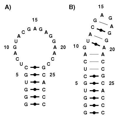
Consider this RNA structure, from the rat 28S rRNA [1], and shown in
Figure 6. This structure features a Sarcin/Ricin motif which is
composed of many non-canonical base pairs [2,3].
|
|
Figure 6. Rat 28S rRNA, featuring the Sarcin/Ricin
motif. a) Classic secondary structure. b) Enhanced
secondary structure.
|
|
One can go on and model the classic secondary structure, using the
techniques described here. However, it is almost improbable that
MC-Sym generates the enhanced structure, with all the non-canonical
base pairs, from modeling with single-stranded stretches. To model a
structure such as Figure 6A, we suggest other alternative programs,
like FARNA [4], which takes into account non-canonical base pairs,
RNA2D3D [5], and iFoldRNA [6].
Classic secondary structures can be further analyzed by MC-Fold for it
to produce enhanced secondary structures. These now could then be
modeled in 3-D more easily using MC-Sym.
|
References:
- Correll et al. PNAS. 1998 95:13436-41.
- Szewczak et al. PNAS. 1993 90:9581-5.
- Wimberly et al. Biochemistry 1993 32:1078-87.
- Das & Baker. PNAS. 2007 104:14664-9.
- Martinez et al. J Biomol Struct Dyn. 2008 25:669-84.
- Ding et al. RNA. 2008 14:1164-73.
|
Several NCM sets are available to the modeler. These sets can be used
in MC-Sym's library command.
- *_t: theoretical set, only for 2_2 NCMs with A=U/C=G base pairs. For example:
ncm_01 = library( pdb( "MCSYM-DB/2_2/UCGA/*_t.pdb.gz" ) ... )
It's purpose is to provide only one 3-D instance for that NCM,
reducing the conformational search space. Useful to model large RNAs,
or to force MC-Sym to sample other parts of the RNA structure. One can
use the R20 sets instead (see below); which would also add the G=U
base pair in a strict set with few, but "high quality", NCMs. Two
problems arise when using the _t sets; 1) consecutive pyrimidines
won't be stacked, at least on the 5' strand. 2) base pairs won't be
propelled.
- *_1: observed set, found in the PDB with the actual sequence. For example:
ncm_01 = library( pdb( "MCSYM-DB/4/GGAA/*_1.pdb.gz" ) ... )
It's purpose is to provide 3-D instances for that NCM that can be
found in the PDB with the actual modeled sequence. Useful to model
parts of an RNA structure which are known to adopt particular folds,
like the GNRA-tetraloops, or base pair steps with proper helical
parameters [1,2,3].
- *_x: artificial set, built from backbone templates. For example:
ncm_01 = library( pdb( "MCSYM-DB/4_2/GUUCGC/*_x.pdb.gz" ) ... )
It's purpose is to provide 3-D instances for that NCM that were built
from a database of backbone templates onto which the flanking base
pairs were fitted, and any other nucleobases added. Useful to model
any NCMs which cannot be found in the PDB. As more nucleotides are
implicated in the NCM, the number of backbone templates diminishes
rapidly. Hence, a user should opt for other modeling options, like modeling internal loops. The artificial set
construction is described in details in [4].
- *_e: energy optimized artificial set, built from backbone templates. For example:
ncm_01 = library( pdb( "MCSYM-DB/2_2/GAGA/*_e.pdb.gz" ) ... )
This set is a subset of *_x, in which each NCM has been
annotated, and only the ones with best energies are kept, for each
suite of base pairs. This set is only available for 2_2 NCMs. This set
is useful to sample many base pair types, but with few instances only
(to keep the search space at minimum).
- *_R*: 2_2 NCMs that come from X-Ray only. For example:
ncm_01 = library( pdb( "MCSYM-DB/2_2/GAGA/*_R*_1.pdb.gz" ) ... )
This set is a subset of *_1, in which each NCM has been solved
with X-Ray. This set is only available for 2_2 NCMs.
- *_Rr*: 2_2 NCMs that come from X-Ray only, with a resolution better or equal to r. For example:
ncm_01 = library( pdb( "MCSYM-DB/2_2/GAGA/*_R20*_1.pdb.gz" ) ... )
This set is a subset of *_R, in which each NCM has been solved
with X-Ray, at a resolution better or equal to r. This set is only
available for 2_2 NCMs. Here, R20 are those NCMs from resolutions
better or equal to 2.0A. Available sets are R10, R15, R20, R25, R30
and R35, for resolutions better or equal to, respectively, 1.0, 1.5,
2.0, 2.5, 3.0 and 3.5 Angstroms. Hence, by using R35, you also use
those lower than 3.5A, that is R30 downto R10. Theoretical NCMs
featuring stacks of Watson-Crick base pairs could be replaced with the
R20 sets, for example. Don't expect to find your favorite 2_2 NCM in
the R10 set though (i.e. solved at a resolution better than 1.0
Angstrom)!
- *: a combination of all other sets. For example:
ncm_01 = library( pdb( "MCSYM-DB/4/UACG/*.pdb.gz" ) ... )
However, MC-Sym will load in that order: 1) the theoretical set (if
any), 2) the observed set (if any), and 3) the artificial set.
|
References:
- Hunter. J Mol Biol. 1993 230:1025-54.
- Hunter. J Mol Biol. 1998 280:407-20.
- Hunter & Lu. J Mol Biol. 1997 265:603-19.
- Parisien & Major. Nature. 2008 452:51-55. Supp Inf
|
In MC-Sym it is possible to model using fragments of RNA 3-D
structures. The NCMs are already an example of modeling with
fragments. Furthermore, user-built fragments can also be used. For
example, consider a base triple built from a previous modeling session
in the working directory key IXYuDpUiAB. You can import this fragment
in the new modeling session using the library command:
triple = library(
	pdb( "../IXYuDpUiAB/*.pdb.gz" ) #1:#2, #3:#5 <- A9:A10, A23:A25
	rmsd( 0.1 sidechain && !( pse || lp || hydrogen ) ) )
One can also load structures from different working directories, like:
triple = library(
	pdb( "../{WorkDir1,WorkDir2,...}/*.pdb.gz" ) #1:#2, #3:#5 <- A9:A10, A23:A25
	rmsd( 0.1 sidechain && !( pse || lp || hydrogen ) ) )
As long as all fragments can map to the desired nucleotide numbering
scheme. This is useful when one wants to embed in a stem an internal
loop which features different base pair patterns, each pattern modeled
individually in their own working directory.
|
|
The transfer RNA molecule is often used as a benchmark for 3-D structure prediction [1]. Here, we use the Yeast tRNA-PHE (PDB code 1EVV) [2] as the 3-D target. Within 24h of computation you should obtain a 3-D model at 4 Angstroms from the crystal structure.
|

|
- The MC-Sym script
- The canonized tRNA 3-D structure, without modified nucleotides
- Superimposed MC-Sym solution (model 2) on crystal (model 1)
|
|
Figure 7. MC-Sym model (blue) superimposed on X-ray crystal structure (gold; PDB file 1EVV). The RMSD of the superposition is 4.0 Angstroms.
|
References:
- Major et al. PNAS. 1993 90:9408-12.
- Jovine et al. J Mol Biol. 2000 301:401-14.
|
|
It is possible to sample an existing RNA 3-D structure using MC-Sym. The trick is to sample each part individually, then assemble the whole molecule from it's sampled parts. This is not quite equivalent to MD or LD, because no energy is implied here, and we make use of "nodes" in the sampled structures (if the sampled parts do not overlap). Here we sample a recently published tRNA, PDB file 2K4C [1].
|

|
- The MC-Sym script which samples the acceptor stem
- The MC-Sym script which samples the anticodon stem/loop
- The MC-Sym script which samples the T stem/loop
- The MC-Sym script which samples the D stem/loop
- The MC-Sym script which assembles the whole tRNA using previous samples
|
|
Figure 8. Superimposed MC-Sym models.
|
References:
- Grishaev et al. J Biomol Nmr. 2008 42:99-109.
|
Modeling large RNAs is possible using MC-Sym. It all boils down to the
number and quality (resolution) of distance constraints; the lesser
the number/quality, the greater the number and diversity of possible
solutions, and hence the time to explore the search space. Basically,
you should:
- Model each stem/hairpin separately.
- Generate many MC-Sym models (change model_limit = 9999).
- use the SCORE + FILTER in the commands.html file,
once all models are generated.
- Model the whole structure using previously built stems/hairpins.
Consider the Modeling with fragments section.
We suggest that you have mastered all aspects of modeling using MC-Sym
before tackling such a task.
WARNING If you do not have distance constraints between your
stems/hairpins then the number of possible 3-D structures is as large
as there are grains of sand on a beach!
|
|
MODELING WITH NMR RESTRAINTS
|
|
|
NMR methods produce distance constraints which in turn can be used in
MC-Sym for it to generate "starting" structures. There are two ways to
exploit the NMR data; the first way is to declare distance constraints
in the MC-Sym script (see the Modeling with
distance constraints section). However, MC-Sym will treat these
distance constraints as "hard", i.e. cannot be violated. Therefore,
these distance constraints must be relaxed for MC-Sym to generate
models.
The other way to exploit the NMR data is to evaluate the fitness of
each MC-Sym model with respect to the NMR restraints. Basically, you
should:
- Generate many MC-Sym models (change model_limit = 9999).
- Use the "NMR" section in the "commands.html" file,
once all
models are generated.
Each MC-Sym model will then be given an NMR violation energy; the
lower the better. The energy is 0 if the distance falls between Dmin
and Dmax, is linear if the distance violation is less than 1 Angstrom,
and is quadratic elsewise. Use "ANALYZE" in the "commands.html" file
to be informed of the many legitimate base pair types for each base
pair steps.
Supported format #1: (example)
    15  GUA H1             19  GUA H1             3.500    6.500
    19  GUA H1             13  URA H3             2.600    5.000
    20  ADE H2             12  GUA H1             2.600    5.000
    20  ADE H2             13  URA H3             1.800    3.600
    20  ADE H2             19  GUA H1             1.800    3.600

123456789012345678901234567890123456789012345678901234567890123456
         1         2         3         4         5         6
Supported format #2: (example)
assign (residue 1 and name H2') (residue 1 and name H3')  2.60  0.78  0.78
assign (residue 1 and name H1') (residue 1 and name H3')  3.20  0.96  0.96
assign (residue 1 and name H3') (residue 1 and name H8)   3.20  0.96  0.96
assign (residue 1 and name H2') (residue 1 and name H8)   4.00  1.20  1.20
assign (residue 1 and name H1') (residue 1 and name H8)   2.90  1.10  1.10
* Other formats may be supported by explicit demand to Dr. Francois Major.
|
|
ADDING FRAGMENTS TO A PARTIAL STRUCTURE
|
|
|
In MC-Sym it is possible to add fragments to a partial structure.
TODO.
|
Installation.
A modeler can download and install MC-Sym locally. However, basic
knowledge of UNIX commands are required. Here are the steps:
- Download MC-Sym from here.
- Install MC-Sym as prescribed.
- Goto the pipeline page here.
- Click on the "snapshot" button of the "What is MC-Sym" section.
- Download your tarball "MCSYM-DB.tar.gz" on your computer.
- Unzip and untar the tarball:
gunzip MCSYM-DB.tar.gz; tar xvf MCSYM-DB.tar
Attention: we suggest to install the tarball in MC-Sym's
folder, i.e. where the MC-Sym executable is found. For example, if you
launch MC-Sym like this: "~/RNA/MC-Sym/mcsym", then install the
tarball in "~/RNA/MC-Sym/". To use the MC-Sym database from a specific
modeling folder, say "~/RNA/Modeling/Hammerhead/" install a UNIX
symbolic link in that folder:
cd ~/RNA/Modeling/Hammerhead/
ln -s MCSYM-DB ~/RNA/MC-Sym/MCSYM-DB/
such that when MC-Sym encounters a "library" command, like:
ncm_01 = library(
      pdb( "MCSYM-DB/4/GGCC/*.pdb.gz" )  ...
then MC-Sym will be able to find it's databases through the symbolic
link. To use MC-Sym:
cd ~/RNA/Modeling/Hammerhead/
~/RNA/MC-Sym/mcsym  ./Hammerhead.mcc
Updating your database.
There will come a time when MC-Sym will produce an error like:
Failed to expand pattern 'MCSYM-DB/4/UACG/*.pdb.gz': No such file or directory
This is because the NCM database is built on-the-fly on our web
server, hence, when you take a snapshot of our database you will not
have those NCMs built subsequently. Since your local version is not
updated automatically you'll have to update your database through
these steps:
- Make a "fake" MC-Sym script with all the "library" commands which fails. For example:
// these are my missing blocks:
library( pdb( "MCSYM-DB/4/UACG/*.pdb.gz" ) )
library( pdb( "MCSYM-DB/4/UCCG/*.pdb.gz" ) )
library( pdb( "MCSYM-DB/4/UGCG/*.pdb.gz" ) )
library( pdb( "MCSYM-DB/4/UUCG/*.pdb.gz" ) )
- Submit this "fake" script to MC-Sym here; wait until the job is queued.
- Refresh your database; repeat steps 3 to 6 of the previous "Installation" section.
To go local or not?
Although running MC-Sym locally has it's advantages, using our web server has also theirs:
- Automatic updates of the NCM database
- Scoring of the 3-D models with an RNA-tailored force-field
- Refinement of the backbones
- Distributed computing facillity
- Analysis of base pair types
|